I recent wrote a post about testing external pointers with finalization in R using C++. The test package is now available at R-Forge for inspiration.
R
Assume that you have created a 3-dim array in R containing vectors of various size: > a<-array(list(),c(2,2,2)) # array where each element contain a numeric vector > a[[1,1,1]]<-rnorm(1) > a[[1,1,2]]<-rnorm(3) > a[[2,1,1]]<-rnorm(2) > a[[2,1,2]]<-rnorm(3) > a[[1,2,1]]<-rnorm(4) > a[[1,2,2]]<-rnorm(3) > a[[2,2,1]]<-rnorm(5) > a[[2,2,2]]<-rnorm(1) > d = dim(a) > d [1] 2 2 2 > i<-1; j<-1; k<-2 > q<-i + j*d[1] + k*(d[1]*d[2]) – (d[1] + d[1]*d[2]) > a[[i,j,k]] # access an element [1] -0.2370040 -0.6009635 3.0550405 > a[[q]] # access the same element using a single index [1] -0.2370040 -0.6009635 3.0550405 Note you can access the array in two ways. Next you want to copy the array to a vector on the C++ side. For instance in a package you may need to do some operations in C++ to speed up time. On the C++ side you can create a function:
I the past days I have been experimenting with how to use R as an interface to an C++ library. I have made a small test package in R that show how it can be done. The idea is to be able to create a C++ object from R and call methods of the C++ class from R before freeing the object from memory in R. The package/function description goes as follows:
It is well known that you can use Sweave to integrate R code into a LaTeX document. However, how do we highlight R code in LaTeX? LaTeX got its own powerful package listings that can highlight source code from various languages. Moreover, the package SweaveListingUtils provides utilities for defining R as a listings “language”. To highlight your R code in your Sweave document you have to include the following code chunk:
Often you need fast access/lookup in R. For instance assume that you have the following data frame/matrix dat >head(dat) x y z [1,] 1 1 1 0.46 -0.89 0.88 -0.21 0.46 0.93 1.06 [2,] 1 1 2 0.72 -0.40 1.71 -0.52 0.95 NA NA [3,] 1 1 3 -0.49 -0.42 -0.26 -0.06 1.07 1.48 1.08 [4,] 1 1 4 -1.55 -0.90 0.15 -0.60 1.86 -1.15 NA [5,] 1 1 5 -0.46 -1.54 -0.40 NA NA NA NA [6,] 1 1 6 0.14 1.13 -2.42 0.86 0.13 -1.60 0.62 x, y and z represent an unique index and the rest of the columns represent a vector. The vectors may be of various length. To find the vector corresponding to index (x,y,z) you can do a normal search:
The last days 5-9 November I have been visiting Professor Anders Ringgaard Kristensen at KU Life. We have been working on a package in R “MDP” which will provide tools for solving Markov decision processes and their extension multi-level hirarchic Markov decision processes. The package will be based on a solver made by Anders in Java.
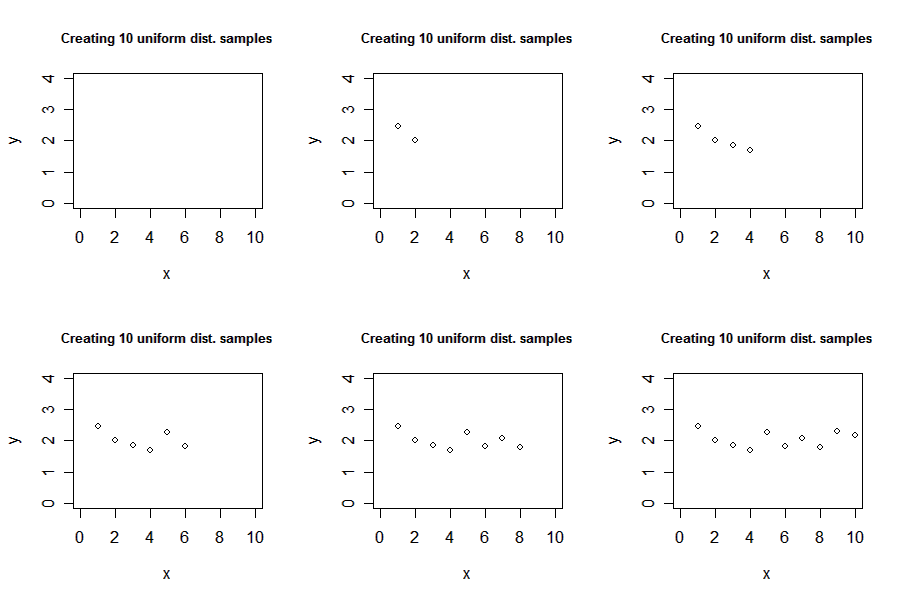
I recent had a discussion with Søren about how one could create an animation of some plots in R. After searching the mail-list it seems that the best way to do it is using ImageMagick which is a free set of tools to create, edit, and compose bitmap images. To use the following guide you must install ImageMagick. Creating an animated gif We create an animated gif file in two steps. First, we save all the plots used in the animation as png files (vector file format) and second, we merge them into a gif animation. Lets try a simple example: > x<-1:10 > y<-runif(10,1.5,2.5) > xlim<-c(0,10) > ylim<-c(0,4) > png(file=”plot%02d.png”, bg=”transparent”) > plot(x, y, type=”n”, xlim=xlim, ylim=ylim) > title(“Create 10 uniform distributed samples”) > for (i in 1:10) plot(x[i], y[i], axes=F, xlab=””, ylab=””, xlim=xlim, ylim=ylim) > dev.off() We have now created intermediate files plot01.png to plot11.png. Note Plot plot01.png […]


